Parsimonious Training
Parsimonious training is the last step (C) of the Auto ML pipeline implemented by Khiops, and consists in selecting the best subset of explicative variables (or aggregates) and weighting them within a Bayesian model:

As an input of this step, the learning algorithm is provided with the encoding models obtained in the previous step (B) for native variables and aggregates making up the root table. The goal of this step is to combine these encodings (discretization or grouping models) in order to build a multivariate predictive model.
Purpose
This section presents the predictive models trained by Khiops in the case of classification. Equivalent models exist for regression problems, for which the interested reader can refer to the published scientific papers. Understanding the MODL approach is a prerequisite, so it is recommended to read the previous sections first.
From Naive to Non-naive Bayes
Khiops provides very competitive models which are both accurate and parsimonious, i.e. selecting very few variables (or aggregates). And yet, these models are derived from the Naïve Bayes classifier which is not exactly recognized for its performance. This section focuses on the important improvements made by Khiops to these models, which are far from being naive 😉.
The big picture
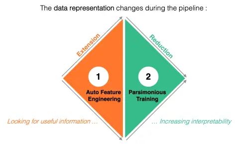
The main idea is illustrated in the following figure, and consists in varying the size of the data representation during the pipeline. Indeed, the Auto Feature Engineering step explores a large number of aggregates which enrich the initial data representation, but which contain redundant information. Next, the parsimonious training step reduces the data representation by selecting a small number of informative and complementary variables. This last step improves model interpretability, as the contributions of selected variables are almost additive since their interactions are reduced to a minimum.
Background
First of all, the expression "Naïve" refers to an hypothesis made about the explicative variables. They are supposed to be independent from each other given the target, which is very rarely the case in real life, hence this pejorative nickname. This assumption is materialized by the red term in the following equation, which shows how is estimated the probability \(p(y_j | \{x_k\}_{k \in [1, K]})\) that a new example \(\{x_k\}_{k \in [1, K]}\) belongs to a particular class \(y_j\):
Indeed, this product is performed on probabilities relative to each explicative variable, which relies on the independence hypothesis. Now, let's take a look at the other important terms:
- The term \(p(y_j)\) is the prior probability of the class \(y_j\). In practice, this term can easily be estimated from the training set, by counting the examples of each class. Here is an illustration:

- The term \(p(x_k|y_j)\) represents the probability of observing a particular value \(x_k\) of the K-th explicative variable, assuming the class to predict is \(y_j\). In practice, this term must be estimated by \(K\) univariate models which can take different forms. The following figure gives two examples. The left part gives the example of parametric distributions (e.g. Gaussian) each fitted on the examples of a given class. The right part shows how discretizations can be used to estimate this term in a frequentist way, by counting the examples of each class within each interval.

- The term \(p(\{x_k\}_{k \in [1, K]})\) represents the probability of observing the example at hand, and is not related to the target variable. To estimate calibrated conditional probabilities, this term can be replaced by the normalization factor represented in blue in the above equation.
Weakness of standard Naïve Bayes
When implemented in an basic way, the Naïve Bayes classifier does not perform very well as the assumption of independence between variables is often not valid in real-life situations. The following weakness needs to be mitigated:
- the term \(p(x_k|y_j)\) is generally not estimated with enough care;
- the dependencies between explicative variables cannot be modeled;
- explicative variables can provide redundant information, which is very bad for performance.
Khiops Brings Major Improvements
Each of these shortcomings is addressed:
#1 : Optimal Encoding
The encoding models (discretization and grouping) are non-parametric estimators, i.e. they can estimate any conditional distribution as long as the number of training examples is sufficient. These models are used to accurately estimate the term \(p(x_k|y_j)\) for each explicative variable.
#2 : Modeling dependencies through aggregates
The Auto Feature Engineering step can produce aggregates which model the dependencies between explicative variables. This is notably the case of the \(Selection\) function, which is able to delimit areas in the input space by using conditions on several variables. For native variables, it is also possible to discretize pairs of variables, and also to train decision trees based on the MODL approach (see publications).
#3 : Fighting information redundancy
Now, we come to the most important improvement which is developed in the rest of this section. As illustrated by the big picture above, a very large number of aggregates can be generated from the Auto Feature Engineering step, which dramatically increases the dimension of the input space. In practice, the construction of the order of \(100,000\) aggregates does not represent a scaling problem. These numerous aggregates are generated independently of each other, exploring the space of aggregates which are informative for predicting the target variable, but without taking any precautions to ensure their independence.
Learning Task of Parsimonious Training
The Parsimonious Training step consists in selecting the subset of variables (native or aggregates) that are both (i) as informative as possible, (ii) and as independent as possible. More specifically, the selected variables are weighted to reduce the effect of their remaining dependencies on the model's performance.
Model Parameters
Khiops implements a robust and well-performing model, called "Selective Non-naive Bayes" (SNB), which takes advantage of the improvements described above (1,2,3) and optimizes variable selection and weighting (4) in the following way:
where \(\{w_k\}_{k \in [1,K]}\) is a vector of weights associated to the \(K\) explicative variables (native or aggregates). These weights are floating-point values such that \(w_k \in [0,1]\), and a large majority of them are null \(w_k = 0\) corresponding to the non-selected variables. This weight vector constitutes the SNB parameters to be optimized during the training process.
Optimization Criterion
As in the other steps of the Auto ML pipeline, the optimization criterion used to learn the SNB model is based on the MODL approach. A variable weighting model \(h\) is entirely defined by the weight vector \(\{w_k\}_{k \in [1,K]}\). And the most probable model given the training set \(d\) is obtained by minimizing the following criterion:
The first two terms correspond to the prior model probability \(-\log(p(h))\), whose distribution is as previously hierarchical and uniform at each level of this hierarchy. Here is the meaning of each term:
- level 1: probability to select a certain number of variables denoted \(K_s\), i.e. the number of non-null weights in the vector \(\{w_k\}_{k \in [1,K]}\). Due to the previous Auto Feature Engineering step, the number of candidate variables (or aggregates) is potentially infinite. Thus, this term represents the probability of choosing \(K_s\) variables from an infinite number. The term \(p^*(K_s)\) is given by the universal Rissanen prior which is the most uniform possible prior on the set of integers. Without going into details, the following figure shows that low values of \(K_s\) are more probable than high values, and the rate of decay is taken to be small as possible.

Key idea #1
The MODL approach is pursued, as the use of the Rissanen prior allows to get as close as possible to a uniform distribution, in order to build a hierarchical and uniform prior distribution.
- level 2: probability of selecting a particular subset of \(K_s\) variables among all possible subsets of the same size, which is derived from a multinomial distribution modeling the selection (or not) of each variable. The term \(p_k\) represents the prior probability of the \(k\)-th selected variable, and is given by the previous Auto Feature Engineering step. Indeed, this term is defined by \(-\log(p_k)=L(h_a^k)+L(h_e^k)\), representing the product of the prior probabilities of the \(k\)-th aggregation model \(h_a^k\) and the \(k\)-th encoding model \(h_e^k\).
Key idea #2
Since the construction cost \(L(h_a^k)\) is taken into account in this prior distribution, the simple aggregates are preferred to complex ones for equivalent likelihoods.
The last term is the negative log-likelihood which measures the quality of the model \(h\) in estimating the target variable of the training data \(d\). It is the sum of the terms \(- \log p(y^{(n)} | \{x^{(n)}_k\}_{k \in [1, K]})\), where \(y^{(n)}\) represents the target value of the \(n\)-th training example and \(\{x^{(n)}_k\}\) its explicative variable values. Finally, the negative log-likelihood evaluates the average quality of the output probabilities estimated by the classifier, since the lower the probability of the true labels, the higher the penalty.
The regularization parameter \(\gamma\) weighs the relative importance of the prior and likelihood terms, so it has an influence on both the parsimony of the trained models and overfitting. Indeed, if \(\gamma = 0\) the optimization criterion is not regularized anymore, which leads to the selection of a large number of variables and to overfitting issues. On the other hand, the choice \(\gamma = 1\) corresponds to a full regularization which makes sense only when the explicative variables are independent. Finally, the use of \(\gamma<1\) is equivalent to relaxing the naïve hypothesis by allowing the selection of additional variables which are not totally independent of the others, and which bring complementary and useful information to improve the model accuracy.
Key idea #3
Khiops does not involve any hyper-parameter, the parameter \(\gamma\) has been adjusted using a large collection of datasets. It is set to a fixed sweet spot value which considerably limits the risks of overfitting in practice and provides parsimonious and accurate models. In addition, the adjustment of this parameter is not very sensitive and does not produce significant variation in accuracy from one data set to another.
Optimization Algorithm
Algorithmic Challenge
This optimizing problem is very hard, since \(\{w_k\}_{k \in [1,K]}\) is a vector of floating-point values, for which there are an infinite number of candidate solutions.
The optimization algorithm used is based on two key principles: (i) for reasons of efficiency, the set of solutions is explored in a discrete way; (ii) in order to prioritize important interactions between variables, the grain level with which the floating-point weights are updated becomes finer and finer.
The following figure illustrates the main steps of this algorithm:
- Step 1 initializes the weight vector \(\{w_k\}\) with zero values, the weight increment is set to \(1\) and the set of selected variables is initialized to the empty set. It is important to keep in mind that the set of selected variables is a working variable, which changes state during the algorithm, and which is used to update the weight vector.
- Step 2 is inspired by the Forward/Backward variable selection algorithm, which attempts to add or remove variables in random order, with the aim of improving the optimization criterion. Then, added variables are used to increment the weight \(w_k\) of the corresponding variables, and similarly deleted variables are used to decrement the weights.
- Step 3 controls the complexity of the algorithm by repeating the previous step a certain number of times, calculated according to the number of available variables and the size of the dataset.
- Step 4 refines the weight vector by repeating the previous steps with decreasing weight increments. This step allows to progressively select variables whose contribution and interaction with the other variables become less and less important.
Technical Benefits
Model Interpretability
The parsimony of the SNB model, which selects a small subset of variables (native or aggregates), combined with the fact that the aggregates generated in the previous Auto Feature Engineering step have explicit names, make the models produced by Khiops very easy to interpret. A visualization tool is provided for this purpose, making it possible to understand and visualize the entire Auto ML pipeline, from optimal encoding to model evaluation.
Fast Predict
The parsimony of the SNB model also represents a major time saver when the model is deployed on large amounts of data. Selecting only a few variables means speed!