Auto Hardware Adaptation
General principles
This section presents the strategy implemented in Khiops for adapting the algorithms to the available hardware resources.
Key idea #1: Divide and conquer
Khiops divides the data into a more or less fine-grained grid of files, depending on the learning task at hand and the available hardware resources.
As shown in the following figure, the successive steps of the Auto ML pipeline are algorithms which process either rows or columns of the root table. For example, optimal encoding is a column-based algorithm, since each discretization or grouping model can be learned independently from each variable (or aggregate). On the other hand, once the pipeline is executed, making predictions is a row-based algorithm, since each example can be scored independently.
The goal is to ensure the proper execution of these algorithms, whatever
- the size of the processed data;
- the amount of available hardware resources.
To do this, Khiops slices the data into a grid of files, each file representing a cell of the grid. Then, these files are grouped into slices, either horizontally for row-based algorithms, or vertically for column-based algorithms.
Key idea #2
A smart strategy adapts the grid size to each situation.
As shown in the following figure, a finer division of the file grid can be decided for two reasons:
- either due to a lack of RAM, with the goal of loading slices in turn into memory and processing them sequentially.
- or due to the availability of numerous CPUs, in order to distribute the processing over the cores of a single computer, or over the workers of a computer cluster (using Message Passing Interface (MPI)).
In practice, this strategy is coded in the following way. At each step of the Auto ML pipeline, the successive algorithms collect more and more precise statistics about the data, and the learning task at hand (the size of the encoding models, the selected variables ...). This information allows each algorithm to estimate its own needs in hardware resources (CPU and RAM), in the worst case and in the best case. The adaptation strategy maps the available resources to the needs of each algorithm and adapts the size of the file grid to each situation. For example, in a non-intuitive way, one should not use too many CPUs to process a small dataset, it is not optimal in terms of computation time. Thus, you are guaranteed that the Auto ML pipeline completes its execution correctly, whatever the hardware resources.
Let's run an experiment!
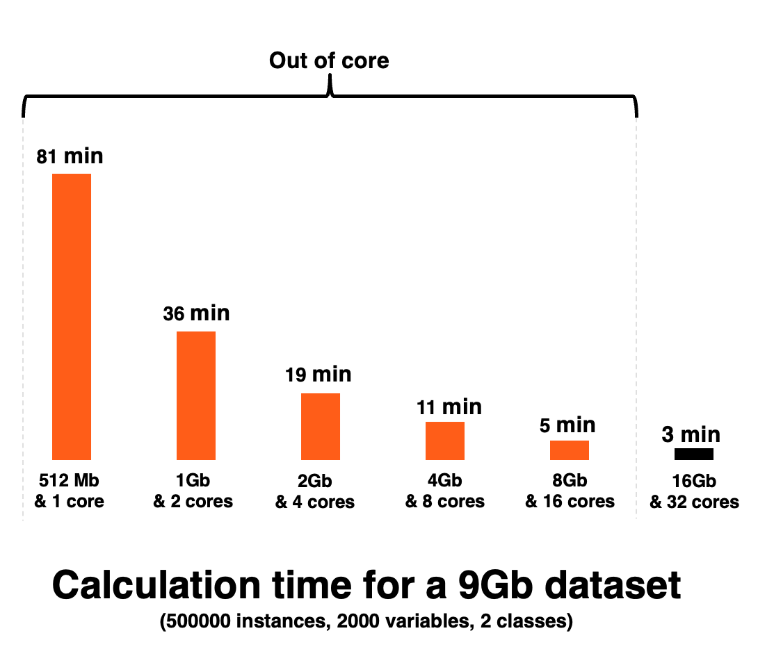
For this experiment, we use the Zeta dataset from the Large Scale Learning Challenge , which contains \(500,000\) training examples and \(2000\) numerical explicative variables. This is a binary classification problem. This data file takes up 9.3 GB on the hard disk, and this run was carried out on a Intel Xeon Gold 6150 CPU 2.70 Ghz. The experiment consists in training a classifier (steps B + C of the pipeline) and evaluating it, by varying the number of cores and the amount of RAM available. 70% of the examples are used for training and 30% for testing.
The following figure plots the execution time in minutes, as the number of cores and the amount of RAM increase together. This figure shows that there is a smooth transition from out-of-core to distributed computing, demonstrating the efficiency of the adaptation strategy to the available hardware resources. This is made possible by thorough I/O optimization. Finally, you won't be penalized significantly if your hardware is undersized for the task at hand. Probably not enough to justify a new investment 😉.

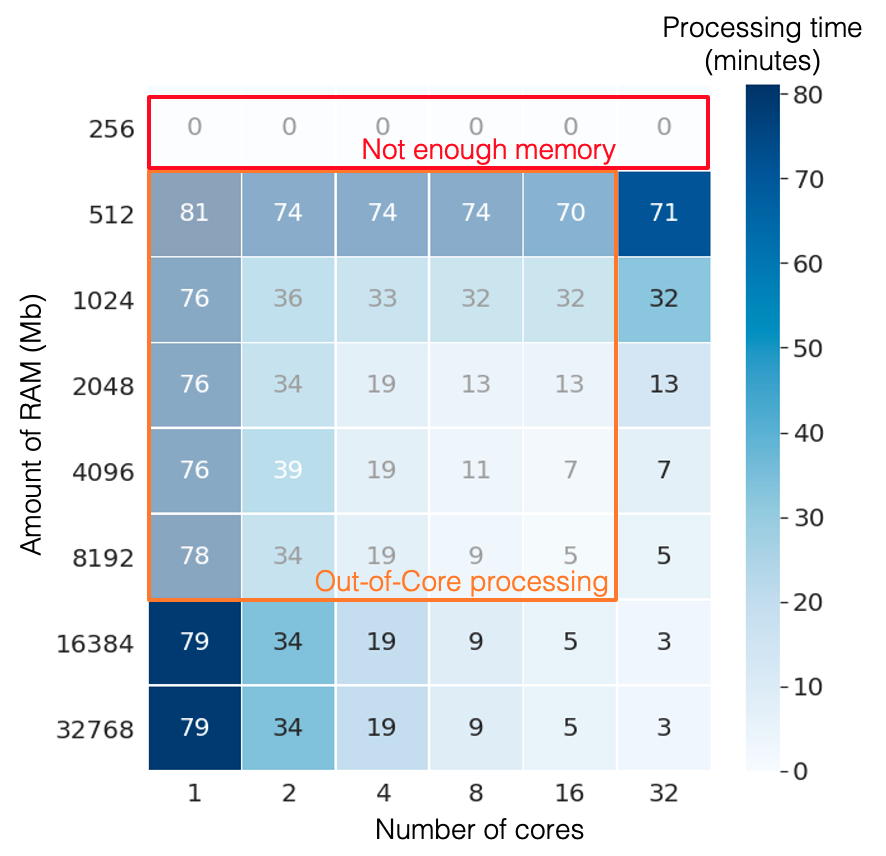
This second more detailed figure shows execution time as a function of the number of cores (horizontal axis) and the amount of RAM available (vertical axis). Out-of-core calculations are represented by the orange rectangle, and once again the transition is smooth on both axes. The red rectangle represents extreme situations where there isn't enough RAM for processing. In this case, Khiops gives an indication of the minimal amount of RAM required to run the process, and above all does not run a long process that will not be completed.

Conclusion
Finally, the computation time is the adjustment variable guaranteeing the proper execution of the algorithms in all situations. In practice, this adaptation strategy allows significant savings: (i) by avoiding investment in additional hardware resources, (ii) by saving engineering time aimed at adapting the code and scaling the training data to the available hardware resources.