Auto Feature Engineering
Multi-table Feature Construction
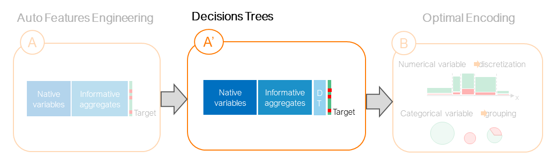
Auto Feature Engineering corresponds to the first (A) step of the Auto-ML pipeline implemented by Khiops. It is an optional pre-processing step to handle multi-table input data. Feature engineering is usually performed manually by data scientists, and is a time-consuming and risky task that can lead to overfitting. Khiops is able to automatically extract a large amount of aggregates from the secondary tables which are constructed and selected to avoid overfitting. These selected aggregates are all informative for the learning task at hand.

In the rest of the pipeline, the aggregates are recoded in step (B), as well as the native variables. Then the encoding models (discretization and univariate grouping) are combined in step (C) in order to learn a parsimonious predictive model, by selecting relatively few variables.
Purpose
This section presents the key ideas of Auto Feature Engineering. For an easier understanding, it is highly recommended to first read the following sections: (i) An original formalism, (ii) Optimal Encoding.
Definition
The Auto Feature Engineering task, also known as propositionalization, consists in "flattening" multi-table data by summarizing the useful information contained in the secondary tables, through new columns inserted in the main table.
Input:
Multi-table data consists of: (i) a root table, where each row represents a training example, (ii) and several secondary tables that potentially contain several records for each example. For example, the customers of a telecommunications company can be described by a root table that contains native variables (name, first name, address, age etc.) and several secondary tables containing detailed information about each customer (contracts, communication details, use of services such as VOD etc). Notice that the target variable is contained in the root table. In our example, this target variable could describe whether a customer is churner or not.
Output:
The purpose of Auto Feature Engineering is to enrich the root table with informative aggregates, which are useful to predict the target variable. These aggregates are computed from the secondary tables. For example, the call rate to a foreign country could be a useful aggregate to predict customer churn. As a result, each row of the enriched root table describes a training example. This table can therefore be used by any learning algorithm.
Key idea #1
Auto Feature Engineering is a supervised learning task that aims at finding the most useful aggregates to predict the target variable.
Model Parameters
As before, the first modeling step is to define the family of models \(\mathcal{H}\) which contains all the learnable hypotheses \(h \in \mathcal{H}\). In the case of Auto Feature Engineering, this family is an extension of the optimal encoding models which perform two tasks: (i) choosing the variable to encode, which can either be a native variable or an aggregate generated from the secondary tables; (ii) encoding this variable by a discretization model or a grouping model depending on its type.
Khiops uses a language similar to SQL to build aggregates. Formally, it is a collection of functions that can be composed with each other an unlimited number of times, provided that the operand and return types of each function are consistent. Here are the main functions used:
| Name | Return type | Operands | Description |
|---|---|---|---|
| \(Count\) | Numerical | Table | Number of records in a table |
| \(CountDistinct\) | Numerical | Table, Categorical | Number of distinct values |
| \(Mode\) | Categorical | Table, Categorical | Most frequent value |
| \(Mean\) | Numerical | Table, Numerical | Mean value |
| \(StdDev\) | Numerical | Table, Numerical | Standard deviation |
| \(Median\) | Numerical | Table, Numerical | Median value |
| \(Min\) | Numerical | Table, Numerical | Min value |
| \(Max\) | Numerical | Table, Numerical | Max value |
| \(Sum\) | Numerical | Table, Numerical | Sum of values |
| \(Selection\) | Table | Table, (Cat, Num) | Selection from a table given a selection criterion |
| \(YearDay\) | Numerical | Date | Day in year |
| \(WeekDay\) | Numerical | Date | Day in week |
| \(DecimalTime\) | Numerical | Time | Decimal hour in day |
In the remainder of this section, we consider a very simple example of multi-table data describing the customers of a company:

The root table contains three columns: (i) the name of the client which is a native categorical variable, (ii) the age of the client which is a native numeric variable, (iii) and the client's identifier which serves as the join key. This key is not an explanatory variable used by the model; it simply identifies the rows of the secondary table corresponding to each client. This multi-table data contains a single secondary table describing the usages of the customers. This table consists of three columns: (i) the join key, (ii) the name of the product used, (iii) and the date of its use.
Here are some examples of aggregates that can be generated from this multi-table data:
- \(Mode\)(Usages, Product)
- \(Max\)(Usages, \(YearDay\)(useDate))
- \(Count\)(\(Selection\)(Usages, \(YearDay\)(useDate) in [1;90] and Product="VOD"))$
Interpretation:
- The first aggregate corresponds to the most frequently used product for each customer,
- The second aggregate combines two functions and represents the day of the year of the last usage,
- The third aggregate is more complex: it corresponds to the number of VOD uses during the first quarter.
Similarly, the aggregates generated by Khiops are named by their formula and can be interpreted by the user.
Key idea #2
The choice of the functions that compose an aggregate and the order in which they are combined are additional parameters which enrich the discretization and grouping models.
As shown in the previous examples, the generated aggregates can be more or less complex, i.e. be composed of a varying number of functions. As the number of compositions is not limited, the aggregates can be arbitrarily complex, which poses a risk of overfitting. This risk is intrinsic to feature engineering, even when it is done manually by data scientists and business experts. For example, to predict customer churn, the following aggregate is certainly too complex to generalize its good performance on test data:
- "the number of calls that a customer makes to Spain, on Friday nights between 10:31 and 10:38, having used the VOD service in the previous 40 minutes".
Key idea #3
The cardinality of the family of models \(\mathcal{H}\) is not bounded, and can potentially be infinite. There is therefore a risk of overfitting and the complexity of the generated aggregates must be regularized.
Optimization Criterion
Information theory provides the same interpretation for both optimization criteria previously described for discretization and grouping models. Indeed, these two criteria can be rewritten as follows:
where the prior term \(L(h)\) refers to the coding length of the model, i.e. the number of bits needed to describe the model parameters. And the likelihood term \(L(d_y | h, d_x)\) is the coding length of the target variable of the training examples \(d_y = \{y_i\}_{i \in [1,n]}\), knowing the model \(h\) and the explanatory variables of the entire training set \(d_x = \{x_i\}_{i \in [1,n]}\). In other words, the encoding model (discretization or grouping) is considered as a compression of the information provided by the target variable of the training set.
In the case of Auto Feature Engineering, the complexity of the aggregates is taken into account in the prior distribution, with a new term \(L(h_a)\), such as:
This term represents a construction cost that penalizes complex aggregates, in order to prevent overfitting. Notice that the model \(h\) is sliced in two, with \(h_a\) representing the constructed aggregate and \(h_e\) being the associated encoding model. The construction cost \(L(h_a)\) is defined recursively, following a hierarchical and uniform prior distribution:
The construction of an aggregate is made according to the following successive choices:
- level 1: generating an aggregate in addition to the \(K\) native variables of the root table is considered as an additional choice, so its probability is \(\frac{1}{K+1}\);
- level 2: the choice of the function is random, the probability of using a particular rule \(\mathcal{R}\) among \(R\) is thus of \(\frac{1}{R}\);
- level 3: each operand of the selected function must be defined, they can be either a variable or the result of another function ...
Notice that \(L(h_a) = \log(K)\) if a native variable is selected instead of generating an aggregate.
Key idea #4
The prior distribution of aggregates has a particular form which prevents overfitting, i.e. it is recursive, hierarchical and uniform. Indeed, there are as many recursions in the prior as there are composed functions, which penalizes complex aggregates. For a complex aggregate to be selected, the additional construction cost in the prior must be compensated by the likelihood, which measures how informative an aggregate is in predicting the target variable.
Sampling Algorithm
Two different algorithms are successively executed to implement Auto Feature Engineering:
- A sampling algorithm which randomly generates aggregates from the prior distribution described above;
- An optimization algorithm which trains the encoding models (discretization or grouping) for each candidate aggregate, and selects only informative ones.
This section describes only (1) the sampling algorithm, as (2) the optimization algorithms for discretization and grouping models are described in the previous section.
Algorithmic Challenge
- How to design an efficient sampling algorithm?
- How to randomly draw aggregates from a family \(\mathcal{H}\) of infinite size, while the hardware resources (RAM and CPU) are limited?
To answer this algorithmic challenge, several heuristics are used:
-
The set of aggregates can be represented in a compact way as a tree, where the branches factorize the successive choices defining the aggregates (i.e. choice of functions to compose, choice of operands). Although compact, this tree has a potentially infinite depth since the number of function compositions is not bounded.
-
Due to limited hardware resources, this tree can only be explored partially. The trick is to use a finite number of tokens that move through the tree and which are distributed on the branches according to the a priori distribution. The tree is thus partially built in RAM, considering only the branches in which tokens circulate.
The animation above shows the sampling algorithm in a very simple case, where the aggregate construction language is limited to three functions (Mode,Min,Max), and where the multi-table data considered is the same as in the previous example. Here is a description of the successive steps:
- Among the \(100\) considered tokens, \(34\) correspond to the choice to generate an aggregate in addition to the two native variables of the root table.
- These \(34\) tokens are uniformly distributed over the \(3\) branches corresponding to the choice of the function to use.
- Then, there is only one possible choice of the 1st operand of these functions, which is the unique secondary table "Usages" of the multi-table data.
- Finally, the last step shows that some branches end (e.g. the function Mode necessarily takes as 2nd operand the categorical variable "Product") and other branches continue to grow through the composition of functions (e.g. the function Min is composed with the function YearDay).
The user specifies a number of candidate aggregates one wants to generate, and the algorithm is repeated several times by increasing the number of tokens, until the wanted number of distinct aggregates is generated. For more details on this sampling algorithm, the interested reader can refer to the scientific publications.
Technical Benefits
Use in any Machine Learning pipeline
Only part of the Khiops Auto ML pipeline can be reused. In particular, the Auto Feature Engineering step can be integrated into any Machine Learning pipeline. This saves a lot of time in data science projects by automatically generating a large number of informative aggregates. Then, any Machine Learning model can be trained from the root table enriched by the aggregates.
Improve business knowledge
The aggregates produced by Khiops are labeled with their mathematical formula, which allows us to interpret them a posteriori. In practice, the analysis of the most informative aggregates allows us to better understand the data and to easily identify the useful information for the learning task at hand.
Decisions Trees
Decision Tree Feature Engineering corresponds to the last (A') step of the Auto-ML pipeline implemented by Khiops. It is an optional pre-processing step to build decisions trees from native variables and aggregates. Khiops is able to automatically build parameter free decisions trees from native variables and informative aggregates.
Definition
A decision tree is a classification model which aims at predicting a categorical class variable from a set of numerical or categorical input variables. One advantage of decision trees is that they provide understandable models, based on decision rules. Khiops exploit a parameter-free Bayesian approach to build decision trees. This approach consist on an analytic formula for the evaluation of the posterior probability of a decision tree given the data. We thus transform the problem into an sampling problem in the space of decision tree models. Khiops build random informative Trees.
Input:
Flat-table data consists of: natives variables and aggregates.
Output:
Informative decision tree
Parameters of the Model
A MODL binary decision tree model is defined by its structure, the distribution of the instances in this structure and the distribution of output values in the leaves. The structure of the decision tree model consists of the set of internal nodes (not leave node), the set of leaves and the relations between these nodes. The distribution of the instances in this structure is defined by the partition of the segmentation variable in each internal node and by the distribution of the classes in each leaf. A decision tree model T is thus defined by:
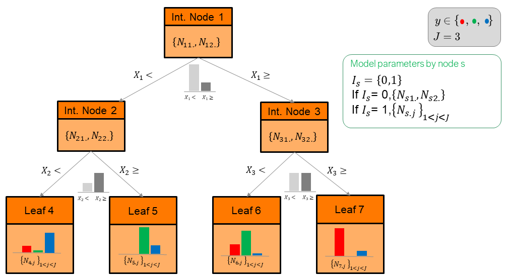
- the subset of variables \(\mathcal{K_T}\) used by model T , that is the number of selected variables \(K_T\) and the choice of the \(K_T\) variables among input set of \(K\) variables,
- the number of child nodes \(I_s\),
- if Is = 0 then the node is an internal node,
- if Is = 1 then the node is a leaf,
- the distribution of the instances in each internal node s:
- the segmentation variable \(X_s\),
- the distribution of the instances on this parts (child nodes) \(\{ N_{s1.},N_{s2.}\}\)
- the distribution of the classes in each leaf l: \(\{N_{l.j} \}_{1≤j≤J}\)
Optimization Criterion
Key idea #1
The MODL decision tree criterion simply result from the expansion of the Bayes' formula.
As MODL discretization the objective of the optimization criterion is to select the most probable model given the training data, denoted \(T\), by maximizing the probability \(P(T|d)=P(T).P(d|T)/P(d)\).
The optimization criterion used to select the most probable supervised decision tree model can easily be interpreted:
The first four terms correspond to the prior model distribution \(-\log(P(T))\), which is hierarchical and uniform at each level of this hierarchy. Here is the meaning of each term:
- level 1: probability of \(K_T\) and probability to select \(K_T\) variables. All the values \(K_T \in [0, K]\) being equiprobable with a probability equals to \(1/(K+1)\), with \(\binom{K + K_T-1}{K_T-1}\) the number of subset of \(K_T\) variables;
- level 2: probability of node \(s\) to split into two nodes according \(X_s\) a numerical variable;
- level 3: probability of node \(s\) to split into two nodes according \(X_s\) a categorical variable, \(B(G_{X_s},2)\) is the number of divisions of the \(G_{X_s}\) values into 2 groups;
- level 4: given the previous parameters of split, probability of observing particular sub-effects by class and by intervals in leave node \(l\), with \(\binom{N_l + J -1}{J-1}\) the number of possible sub-effects.
The last term represents the Likelihood \(-\log(P(d|T))\) which enumerates the training sets that can be generated such that they are correctly described by the model. It is calculated by counting the permutations of the training examples within each leave (numerator) and the permutations of the labels (denominator). Note that the groups of examples located in each leave are considered to be independent (i.e. the sum corresponds to a probability product), which is the case when the training examples are i.i.d (independent and identically distributed), as always in Machine Learning.
Random Trees Generation
The purpose of this section is to introduce the intuitions of the Random trees generation, for more details, you can refer to scientific publications.
Khiops doesn't search to build best tree according to the decision tree criterion. The induction of an optimal decision tree from a data set is NP-hard. The exhaustive search algorithm is then excluded. We use an approximate criterion to generate random informative decision trees. To do this, we exploit a pre-pruning algorithm on a random subsample of \(K_T\) variables (\(K_T=\sqrt K\)). The pre-pruning algorithm starts with the root node and searches for all the partitions from the \(K_T\) variables that improve the criterion. We choose randomly a partition and the leaf is split. For each leaf, the partition is performed according to the univariate MODL discretization or grouping methods, then the global cost of the tree is updated by accounting for this new partition. The algorithm continues to split the leaves until there are no more partitions that improve the tree criterion.